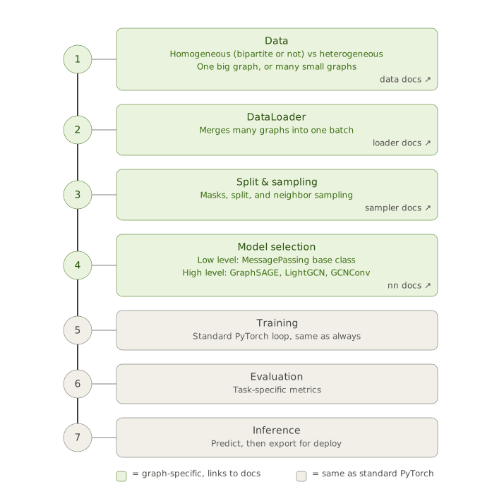
📊 What Do We Expect from a Mature Deep Learning Library?

PyTorch Geometric (PyG): From Prototyping to Enterprise Production

🌐 1. Active Community & World-Class Documentation

Thriving Open Source Community: ~24,000 GitHub stars & 4,000+ forks. The latest PyG 2.7 release alone had 53 contributors across 282+ commits. Active official Slack. Not a dead academic repo—ships monthly!
Exhaustive Documentation: Full ReadTheDocs site with dedicated tutorials for every subsystem (sampling, distributed training, explainability, compilation).

🚀 2. Production Scalability & Out-of-Memory (OOM) Scaling

Distributed & Multi-GPU Training:
- torch_geometric.distributed (v2.5+) — Built for multi-node graphs larger than single-machine RAM using graph partitioning + DDP.
- Plain multi-GPU via standard DistributedDataParallel.
Large-Graph Subgraph Sampling: NeighborLoader, ClusterGCN, and Hierarchical Neighborhood Sampling (trims subgraphs before each GNN layer).
Remote Backends: FeatureStore & GraphStore plug straight into external graph databases or vector stores—skipping expensive ETL steps.

🛠️ 3. Architecture, API & Compiler Stack

Dual-Tier API: High-level modular layers (GCNConv, GraphSAGE, HGTConv) vs. low-level MessagePassing base class for custom aggregation logic.
Heterogeneous Graph Support: First-class native support for multi-entity graphs (HeteroData) using specialized layers like HGTConv and HANConv.
Config-Driven Sweeps (GraphGym): Run YAML-defined experiment sweeps across dozens of architectures via torch_geometric.graphgym.
Compiler & Interpretability:
- Explainability: torch_geometric.explain (supports GNNExplainer, PGExplainer, & Captum).
- JIT & Compile: Direct torch.jit.script() support (v2.5+) and PyG-optimized torch_geometric.compile().

🤖 4. The Cutting-Edge Frontier: GNN + LLM (`torch_geometric.llm`)

TXT2KG: Automated Knowledge Graph construction directly from unstructured raw text.
G-Retriever: Graph-Augmented Generation (Graph-RAG) over structured knowledge graphs.
GLEM: Joint co-training of Large Language Models and GNNs on text-attributed graphs.
RAGQueryLoader: Fetches relevant query subgraphs on the fly from remote backends.

📁 PyG Documentation | Official PyG GitHub Examples

Training EcoSystem

gnn_training

📊 Core PyG Primitive — `torch_geometric.data.Data`

How PyG Represents Homogeneous Graphs in Memory

A single graph in PyG is modeled by the Data class. It encapsulates nodes, pairwise connections (edges), and their associated features/targets across three granularities: node-level, edge-level, and graph-level.

🧩 Core Attributes Breakdown

Attribute	Tensor Shape	Data Type	Description
`data.x`	`[num_nodes, num_node_features]`	`torch.float`	Node Feature Matrix: Holds node representations (e.g., embeddings, tabular features, or node IDs).
`data.edge_index`	`[2, num_edges]`	`torch.long`	Graph Connectivity: Represents source \(\rightarrow\) target edges in Sparse COO Format.
`data.edge_attr`	`[num_edges, num_edge_features]`	`torch.float`	Edge Feature Matrix: Edge weights, interaction timestamps, or rating types.
`data.y`	Arbitrary Shape	Varies	Target Labels: Node targets (`[num_nodes, ]`), graph targets (`[1, ]`), or edge targets.

⚡ Critical Concept: The COO Format (`edge_index`)

⚠️ Common Developer Pitfall: edge_index is shape [2, num_edges], NOT [num_edges, 2].

PyG uses PyTorch’s Coordinate Format (COO) to represent sparse graph connections efficiently: * Row 0 (edge_index[0]): Array of Source Node IDs * Row 1 (edge_index[1]): Array of Target Node IDs

Code

import torch
TORCH = torch.__version__.split('+')[0]
CUDA = 'cu' + torch.version.cuda.replace('.', '') if torch.version.cuda else 'cpu'
print(TORCH, CUDA)
!pip install -q torch_geometric umap-learn plotly
print("pytorch geometric installation done")
!pip install  -q pyg_lib torch_scatter torch_sparse -f https://data.pyg.org/whl/torch-{TORCH}+{CUDA}.html
print('Bunch of extra pytorch dependencies installation done')

2.11.0 cpu

pytorch geometric installation done

     ━━━━━━━━━━━━━━━━━━━━━━━━━━━━━━━━━━━━━━━━ 2.4/2.4 MB 25.0 MB/s eta 0:00:00

     ━━━━━━━━━━━━━━━━━━━━━━━━━━━━━━━━━━━━━━ 681.6/681.6 kB 33.3 MB/s eta 0:00:00

     ━━━━━━━━━━━━━━━━━━━━━━━━━━━━━━━━━━━━━━━━ 1.4/1.4 MB 24.3 MB/s eta 0:00:00

Bunch of extra pytorch dependencies installation done

📊 PyG Data Structures in Practice

Homogeneous (Data) vs. Heterogeneous (HeteroData) Graphs

💡 What’s the Difference?

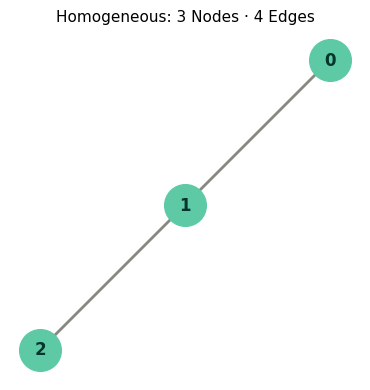
Homogeneous Graph (Data): All nodes belong to a single entity type (e.g., all users or all molecules) and all edges represent one relationship type.
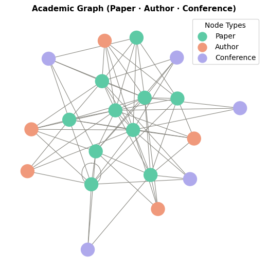
Heterogeneous Graph (HeteroData): Contains multiple distinct node types (e.g., Paper, Author, Conference) and multiple relation types (e.g., cites, writes).

Code

import torch
import networkx as nx
import matplotlib.pyplot as plt
from torch_geometric.data import Data, HeteroData
from torch_geometric.utils import to_networkx

# Set seed for reproducibility
torch.manual_seed(42)
device = torch.device('cuda' if torch.cuda.is_available() else 'cpu')

# ==============================================================================
# 1. HOMOGENEOUS GRAPH (`Data`)
# ==============================================================================
edge_index = torch.tensor([
    [0, 1, 1, 2],
    [1, 0, 2, 1]
], dtype=torch.long)

x = torch.tensor([[-1.0], [0.0], [1.0]], dtype=torch.float)

homo_data = Data(x=x, edge_index=edge_index).to(device)

print("="*50)
print(" 🟢 HOMOGENEOUS GRAPH INSPECTION ")
print("="*50)
print(f"Graph Representation : {homo_data}")
print(f"Data Keys            : {homo_data.keys()}")
print(f"Nodes / Edges        : {homo_data.num_nodes} Nodes | {homo_data.num_edges} Edges")
print(f"Features Per Node    : {homo_data.num_node_features}")
print(f"Has Isolated Nodes?  : {homo_data.has_isolated_nodes()}")
print(f"Has Self-Loops?      : {homo_data.has_self_loops()}")
print(f"Is Directed Graph?   : {homo_data.is_directed()}\n")

# Plot Homogeneous Graph
G_homo = to_networkx(homo_data.cpu(), to_undirected=True)
pos_homo = nx.spring_layout(G_homo, seed=42)

plt.figure(figsize=(3.5, 3.5))
nx.draw(
    G_homo, pos_homo,
    with_labels=True,
    node_color='#5DCAA5',
    node_size=900,
    font_size=12,
    font_weight='bold',
    font_color='#04342C',
    edge_color='#888780',
    width=2
)
plt.title(f'Homogeneous: {homo_data.num_nodes} Nodes · {homo_data.num_edges} Edges', fontsize=11)
plt.axis('off')
plt.show()

# ==============================================================================
# 2. HETEROGENEOUS GRAPH (`HeteroData`)
# ==============================================================================
hetero_data = HeteroData()

# Node Features per Type
hetero_data['paper'].x = torch.randn(10, 16)       # 10 Papers, 16 features
hetero_data['author'].x = torch.randn(5, 32)       # 5 Authors, 32 features
hetero_data['conference'].x = torch.randn(5, 8)    # 5 Conferences, 8 features

# Edges per Relation
hetero_data['paper', 'cities', 'paper'].edge_index = torch.randint(0, 10, (2, 50))

hetero_data['author', 'paper'].edge_index = torch.stack([
    torch.randint(0, 5, (30,)),
    torch.randint(0, 10, (30,))
])

hetero_data['paper', 'conference'].edge_index = torch.stack([
    torch.randint(0, 10, (25,)),
    torch.randint(0, 5, (25,))
])

hetero_data = hetero_data.to(device)

print("\n" + "="*50)
print(" 🟣 HETERO GRAPH INSPECTION ")
print("="*50)
print(hetero_data)
print("\nSample Relation Lookup ('author', 'to', 'paper'):")
print(hetero_data['author', 'to', 'paper'].edge_index[:, :5])

# Plot Heterogeneous Graph
def plot_hetero_graph(hdata, title="Academic Graph (Paper · Author · Conference)"):
    homo = hdata.cpu().to_homogeneous()
    G_hetero = to_networkx(homo, to_undirected=True)
    pos_hetero = nx.spring_layout(G_hetero, seed=42)

    palette = {0: '#5DCAA5', 1: '#F0997B', 2: '#AFA9EC'}
    node_colors = [palette[t] for t in homo.node_type.tolist()]

    plt.figure(figsize=(5, 5))
    nx.draw(
        G_hetero, pos_hetero,
        node_color=node_colors,
        node_size=350,
        edge_color='#888780',
        width=0.8
    )

    for t, node_type in enumerate(hdata.node_types):
        plt.scatter([], [], c=palette[t], label=node_type.capitalize(), s=150)

    plt.legend(frameon=True, loc='upper right', title="Node Types")
    plt.title(title, fontsize=11, fontweight='bold')
    plt.axis('off')
    plt.show()

plot_hetero_graph(hetero_data)

==================================================
 🟢 HOMOGENEOUS GRAPH INSPECTION 
==================================================
Graph Representation : Data(x=[3, 1], edge_index=[2, 4])
Data Keys            : ['x', 'edge_index']
Nodes / Edges        : 3 Nodes | 4 Edges
Features Per Node    : 1
Has Isolated Nodes?  : False
Has Self-Loops?      : False
Is Directed Graph?   : False


==================================================
 🟣 HETERO GRAPH INSPECTION 
==================================================
HeteroData(
  paper={ x=[10, 16] },
  author={ x=[5, 32] },
  conference={ x=[5, 8] },
  (paper, cites, paper)={ edge_index=[2, 50] },
  (author, to, paper)={ edge_index=[2, 30] },
  (paper, to, conference)={ edge_index=[2, 25] }
)

Sample Relation Lookup ('author', 'to', 'paper'):
tensor([[1, 4, 0, 4, 0],
        [3, 6, 3, 5, 4]])

📊 Slide 4: Real-World Graph Prep — MovieLens-100K

Translating Recommendation Data into a Unified GNN Graph

🎬 About the Dataset

Source: Benchmark MovieLens-100K dataset containing 100,000 rating interactions.
Nodes: 943 Users and 1,682 Movies (Total: 2,625 Nodes).
Graph Type: Naturally a Bipartite Graph (Users connect only to Movies, Movies connect only to Users).

💡 Key Modeling Assumptions & Transformations

Implicit Feedback Assumption:
- We discard explicit 1–5 star ratings and treat any rating as a binary interaction signal (\(1 = \text{interaction happened}\)).
- Simplifies the system to learn general user preference retrieval rather than rating regression.
Homogeneous Graph Unification (The “ID-Shift Trick”):
- Instead of managing complex multi-type dictionaries (HeteroData), we unify Users and Movies into a single continuous index space:
  - User Node IDs: \(0 \dots 942\)
  - Movie Node IDs: \(943 \dots 2,624\) (shifted by \(+943\))
- Why? Allows us to feed raw node IDs directly into a standard PyTorch nn.Embedding(2625, dim) layer to learn representations from scratch!
Bidirectional Message Passing:
- Interaction edges are mirrored (\(User \rightarrow Movie\) and \(Movie \rightarrow User\)).
- \(100,000 \text{ raw interactions} \times 2 = \mathbf{200,000 \text{ total directed edges}}\).
- Ensures GNN message-passing information flows seamlessly in both directions during convolution.

Code

import torch
from torch_geometric.data import Data
from torch_geometric.datasets import MovieLens100K

# Set random seed for reproducibility
torch.manual_seed(42)
device = torch.device('cuda' if torch.cuda.is_available() else 'cpu')

# ==============================================================================
# 1. LOAD MOVIELENS DATASET
# ==============================================================================
dataset = MovieLens100K(root='./data/MovieLens100K')
data = dataset[0]

no_user_nodes = data['user'].num_nodes     # 943 Users
no_movie_nodes = data['movie'].num_nodes   # 1,682 Movies
total_nodes = no_user_nodes + no_movie_nodes # 2,625 Total Nodes

# ==============================================================================
# 2. COMBINE & SHIFT INDEXES INTO HOMOGENEOUS SPACE
# ==============================================================================
# Combine train and test interactions back into the full 100K interaction graph
edge_index = torch.cat([
    data['user', 'rates', 'movie'].edge_index,
    data['user', 'rates', 'movie'].edge_label_index,
], dim=1)

# Shift Movie IDs past User IDs -> Movie IDs start at index 943
edge_index[1] = edge_index[1] + no_user_nodes

# Add reverse direction (Movie -> User) for 2-way message passing
edge_index = torch.cat([edge_index, edge_index.flip(0)], dim=1)

# ==============================================================================
# 3. BUILD UNIFIED PyG DATA OBJECT
# ==============================================================================
movielens_data = Data(
    x=torch.arange(total_nodes), # Global node IDs [0 ... 2624]
    edge_index=edge_index,
).to(device)

print("="*50)
print(" 🎬 MOVIELENS-100K HOMOGENEOUS GRAPH SUMMARY ")
print("="*50)
print(f"Total Unique Nodes : {movielens_data.num_nodes} ({no_user_nodes} Users + {no_movie_nodes} Movies)")
print(f"User Index Range   : [0 ... {no_user_nodes - 1}]")
print(f"Movie Index Range  : [{no_user_nodes} ... {total_nodes - 1}]")
print(f"Bidirectional Edges: {movielens_data.num_edges} edges")
print(f"PyG Data Object    : {movielens_data}")

==================================================
 🎬 MOVIELENS-100K HOMOGENEOUS GRAPH SUMMARY 
==================================================
Total Unique Nodes : 2625 (943 Users + 1682 Movies)
User Index Range   : [0 ... 942]
Movie Index Range  : [943 ... 2624]
Bidirectional Edges: 200000 edges
PyG Data Object    : Data(x=[2625], edge_index=[2, 200000])

Code

data

HeteroData(
  movie={ x=[1682, 18] },
  user={ x=[943, 24] },
  (user, rates, movie)={
    edge_index=[2, 80000],
    rating=[80000],
    time=[80000],
    edge_label_index=[2, 20000],
    edge_label=[20000],
  },
  (movie, rated_by, user)={
    edge_index=[2, 80000],
    rating=[80000],
    time=[80000],
  }
)

Code

import torch
import torch_geometric.transforms as T
from torch_geometric.datasets import MovieLens100K

# Set random seed for reproducibility
torch.manual_seed(42)
device = torch.device('cuda' if torch.cuda.is_available() else 'cpu')

# ==============================================================================
# 1. LOAD MOVIELENS DATASET (Natively loads as HeteroData)
# ==============================================================================
dataset = MovieLens100K(root='./data/MovieLens100K')
data = dataset[0]
print(data)
no_user_nodes = data['user'].num_nodes     # 943 Users
no_movie_nodes = data['movie'].num_nodes   # 1,682 Movies

# ==============================================================================
# 2. COMBINE FULL INTERACTIONS (User -> Movie)
# ==============================================================================
# Merge raw train/test edge splits back into one full interaction matrix
full_edge_index = torch.cat([
  data['user', 'rates', 'movie'].edge_index,
  data['user', 'rates', 'movie'].edge_label_index,
], dim=1)
data['user', 'rates', 'movie'].edge_index = full_edge_index

# Clean up raw label attributes before performing RandomLinkSplit later
if hasattr(data['user', 'rates', 'movie'], 'edge_label_index'):
  del data['user', 'rates', 'movie'].edge_label_index
  del data['user', 'rates', 'movie'].rating
  del data['user', 'rates', 'movie'].time
if hasattr(data['user', 'rates', 'movie'], 'edge_label'):
  del data['user', 'rates', 'movie'].edge_label
del data['movie', 'rated_by', 'user']

# ==============================================================================
# 3. SET INDEPENDENT NODE ID FEATURES
# ==============================================================================
# Each node type gets its own zero-indexed ID array [0 ... N-1]
data['user'].x = torch.arange(no_user_nodes)
data['movie'].x = torch.arange(no_movie_nodes)

# ==============================================================================
# 4. ADD REVERSE EDGES AUTOMATICALLY ('movie', 'rev_rates', 'user')
# ==============================================================================
# T.ToUndirected() creates the reverse bipartite edges for 2-way message passing
movielens_data = T.ToUndirected()(data).to(device)

# ==============================================================================
# 5. INSPECT HETEROGENEOUS GRAPH STRUCTURE
# ==============================================================================
print("="*60)
print(" 🎬 MOVIELENS-100K HETEROGENEOUS GRAPH SUMMARY ")
print("="*60)
print(f"User Nodes  ('user')  : {movielens_data['user'].num_nodes} nodes [Index Range: 0 ... {no_user_nodes - 1}]")
print(f"Movie Nodes ('movie') : {movielens_data['movie'].num_nodes} nodes [Index Range: 0 ... {no_movie_nodes - 1}]")
print("-" * 60)
print(f"Forward Edges ('user', 'rates', 'movie')    : {movielens_data['user', 'rates', 'movie'].num_edges} edges")
print(f"Reverse Edges ('movie', 'rev_rates', 'user'): {movielens_data['movie', 'rev_rates', 'user'].num_edges} edges")
print("="*60)
print("\nPyG HeteroData Object Representation:")
print(movielens_data)

HeteroData(
  movie={ x=[1682, 18] },
  user={ x=[943, 24] },
  (user, rates, movie)={
    edge_index=[2, 80000],
    rating=[80000],
    time=[80000],
    edge_label_index=[2, 20000],
    edge_label=[20000],
  },
  (movie, rated_by, user)={
    edge_index=[2, 80000],
    rating=[80000],
    time=[80000],
  }
)
============================================================
 🎬 MOVIELENS-100K HETEROGENEOUS GRAPH SUMMARY 
============================================================
User Nodes  ('user')  : 943 nodes [Index Range: 0 ... 942]
Movie Nodes ('movie') : 1682 nodes [Index Range: 0 ... 1681]
------------------------------------------------------------
Forward Edges ('user', 'rates', 'movie')    : 100000 edges
Reverse Edges ('movie', 'rev_rates', 'user'): 100000 edges
============================================================

PyG HeteroData Object Representation:
HeteroData(
  movie={ x=[1682] },
  user={ x=[943] },
  (user, rates, movie)={ edge_index=[2, 100000] },
  (movie, rev_rates, user)={ edge_index=[2, 100000] }
)

📊 Link Prediction Splitting with `RandomLinkSplit`

How to Split Graph Edges Without Causing Data Leakage

🤔 Why Can’t We Use Standard `train_test_split`?

In traditional ML, splitting data means randomly picking rows. In Graph Link Prediction, this breaks everything: * Data Leakage Risk: If a test edge remains inside data.edge_index, your GNN will perform message passing directly across the target edge during forward propagation—effectively letting the model “cheat” and read the answer. * The Solution: RandomLinkSplit decouples the graph into two distinct edge sets per split: 1. edge_index (Message Passing Graph): The structural graph used to aggregate neighbor features. 2. edge_label_index (Supervision Targets): The specific pairs we predict and compute loss against.

🎨 Visual Mechanism of `RandomLinkSplit`

⚙️ Important Parameter Breakdown

num_val=0.0 & num_test=0.2: Instructs PyG to perform a strict 80% Train / 20% Test split, removing the validation stage entirely.
is_undirected=True: Crucial for symmetric graphs. Guarantees that if edge \((u \rightarrow v)\) is removed for testing, its reverse twin \((v \rightarrow u)\) is also removed, completely sealing information leaks.
add_negative_train_samples=False: Prevents static negative pair generation during the split. Leaves negative edge generation to the LinkNeighborLoader dynamically per batch.

Code

import torch
from torch_geometric.transforms import RandomLinkSplit

# Set random seed for reproducibility
torch.manual_seed(42)

# ==============================================================================
# 1. DEFINE RANDOM LINK SPLIT (Train / Test Split Only)
# ==============================================================================
transform = RandomLinkSplit(
    num_val=0.0,                        # Remove validation set (0% Val)
    num_test=0.2,                       # 20% held-out test edges
    add_negative_train_samples=False,   # Handled dynamically by LinkNeighborLoader
    edge_types=[('user', 'rates', 'movie')],
    rev_edge_types=[('movie', 'rev_rates', 'user')]

)

# ==============================================================================
# 2. EXECUTE THE SPLIT ON MOVIELENS DATA
# ==============================================================================
train_data, val_data, test_data = transform(movielens_data)
print(train_data)

# Shortcut variable for the primary supervision relation
target_rel = ('user', 'rates', 'movie')

# ==============================================================================
# 3. VERIFY TENSOR SHAPES & HETEROGENEOUS RELATIONAL ATTRIBUTES
# ==============================================================================
print("="*65)
print(" ✂️ HETEROGENEOUS RANDOM LINK SPLIT SUMMARY ")
print("="*65)
print(f"Original Forward Edges ('user','rates','movie') : {movielens_data[target_rel].num_edges}")
print("-" * 65)
print(f"Train Message-Passing Edges                     : {train_data[target_rel].edge_index.shape}")
print(f"Train Target Supervision Pairs                  : {train_data[target_rel].edge_label_index.shape}")
print(f"Train Label Distribution                        : {torch.bincount(train_data[target_rel].edge_label.int()).tolist()} (All 1.0 Positives)")
print("-" * 65)
print(f"Test Message-Passing Edges                      : {test_data[target_rel].edge_index.shape}")
print(f"Test Target Supervision Pairs                   : {test_data[target_rel].edge_label_index.shape}")
print(f"Test Label Distribution                         : {torch.bincount(test_data[target_rel].edge_label.int()).tolist()} (50% Pos / 50% Neg)")
print("="*65)

HeteroData(
  movie={ x=[1682] },
  user={ x=[943] },
  (user, rates, movie)={
    edge_index=[2, 80000],
    edge_label=[80000],
    edge_label_index=[2, 80000],
  },
  (movie, rev_rates, user)={ edge_index=[2, 80000] }
)
=================================================================
 ✂️ HETEROGENEOUS RANDOM LINK SPLIT SUMMARY 
=================================================================
Original Forward Edges ('user','rates','movie') : 100000
-----------------------------------------------------------------
Train Message-Passing Edges                     : torch.Size([2, 80000])
Train Target Supervision Pairs                  : torch.Size([2, 80000])
Train Label Distribution                        : [0, 80000] (All 1.0 Positives)
-----------------------------------------------------------------
Test Message-Passing Edges                      : torch.Size([2, 80000])
Test Target Supervision Pairs                   : torch.Size([2, 40000])
Test Label Distribution                         : [20000, 20000] (50% Pos / 50% Neg)
=================================================================

Code

test_data

HeteroData(
  movie={ x=[1682] },
  user={ x=[943] },
  (user, rates, movie)={
    edge_index=[2, 80000],
    edge_label=[40000],
    edge_label_index=[2, 40000],
  },
  (movie, rev_rates, user)={ edge_index=[2, 80000] }
)

Mini-Batch Subgraph Sampling via `LinkNeighborLoader`

Scaling Graph Neural Networks Beyond Full-Graph In-Memory Limitations

🚀 The Full-Graph Scalability Bottleneck

In full-graph training, every single GNN forward pass processes the entire adjacency matrix (\(\mathbf{A} \in \mathbb{R}^{|V| \times |V|}\)). For real-world graphs with millions of users and items, this causes immediate Out-Of-Memory (OOM) errors on GPU devices.

LinkNeighborLoader solves this through localized mini-batch neighborhood sampling: 1. Seed Selection: Selects a mini-batch of target supervision edges from edge_label_index. 2. Dynamic Negative Sampling: If configured, generates unobserved negative target pairs on-the-fly. 3. \(k\)-Hop Expansion: Recursively samples a bounded number of neighbors around the seed nodes layer by layer (\(N_1, N_2, \dots, N_L\)). 4. Subgraph Extraction & Relabeling: Extracts the localized induced subgraph and relabels global node IDs into contiguous local indices (\(0 \dots N_{\text{subgraph}}-1\)).

🎨 Visualizing 1 Iteration of Subgraph Extraction

🔍 Anatomy of 1 Mini-Batch Iteration Output

When executing batch = next(iter(train_loader)), PyG returns a localized data container holding four vital tensors:

batch.n_id \(\to\) [Num_Subgraph_Nodes]
- Vector of Global Node IDs included inside this specific sampled neighborhood subgraph.
- Used to index global node feature matrices or embedding lookup tables: x_sub = model.embedding(batch.n_id).
batch.edge_index \(\to\) [2, Num_Subgraph_Edges]
- Sparse adjacency matrix representing message-passing connectivity strictly within the sampled subgraph.
- Local Relabeling: Indices are mapped into range \([0 \dots N_{\text{subgraph}}-1]\) so standard PyG convolution layers function seamlessly.
batch.edge_label_index \(\to\) [2, Num_Target_Pairs]
- Local node index pairs representing the supervision target edges (both positive and negative pairs) for loss computation.
batch.edge_label \(\to\) [Num_Target_Pairs]
- Binary floating-point targets (\(1.0\) for ground-truth interactions, \(0.0\) for sampled non-interactions).

⚙️ Training Loader vs. Testing Loader Strategy

Configuration Parameter	`train_loader`	`test_loader`	Strategic Technical Reason
`data` Source	`train_data`	`test_data`	Evaluates models on unseen test split graphs.
`num_neighbors`	`[20, 10]`	`[20, 10]`	Bounds computational fan-out to \(20\) 1-hop and \(10\) 2-hop neighbors.
`batch_size`	`1024` or `2048`	`1024` or `2048`	Number of seed supervision target edges per mini-batch.
`neg_sampling_ratio`	`1.0`	`0.0`	Train: Dynamically samples \(1\) random negative per positive edge per epoch. Test: Set to `0.0` because `test_data` already holds static negative pairs.
`shuffle`	`True`	`False`	Randomizes batch order during training; preserves deterministic evaluation order during testing.

💻

Code

import torch
from torch_geometric.loader import LinkNeighborLoader

# Set seed for reproducibility
torch.manual_seed(42)

# Shortcut variable for the target supervision edge type
target_rel = ('user', 'rates', 'movie')

# ==============================================================================
# 1. BUILD HETERO TRAIN LOADER (Dynamic Bipartite Negative Sampling)
# ==============================================================================
train_loader = LinkNeighborLoader(
    data=train_data,
    num_neighbors=[20, 10],                 # 20 1-hop, 10 2-hop neighbors sampled per relation
    batch_size=1024,                        # 1024 seed positive target edges
    edge_label_index=(target_rel, train_data[target_rel].edge_label_index),
    edge_label=train_data[target_rel].edge_label,
    neg_sampling_ratio=1.0,                 # Dynamically samples 1 negative Movie per User pair
    shuffle=True
)

# ==============================================================================
# 2. BUILD HETERO TEST LOADER (Static Pre-Allocated Negatives)
# ==============================================================================
test_loader = LinkNeighborLoader(
    data=test_data,
    num_neighbors=[20, 10],                 # Identical neighborhood fan-out
    batch_size=1024,                        # Seed target pairs per test batch
    edge_label_index=(target_rel, test_data[target_rel].edge_label_index),
    edge_label=test_data[target_rel].edge_label,
    neg_sampling_ratio=0.0,                 # 0.0 because test_data already possesses static negatives
    shuffle=False
)

# ==============================================================================
# 3. INSPECT EXACTLY 1 HETERO MINI-BATCH ITERATION
# ==============================================================================
# Fetch the very first mini-batch iteration from train_loader
first_batch = next(iter(train_loader)).to(device)

print("="*65)
print(" 🔬 DECONSTRUCTING 1 ITERATION OF Hetero LinkNeighborLoader ")
print("="*65)
print(f"Mini-Batch HeteroData Representation : {first_batch}")
print("-" * 65)
print("1. Subgraph Node Identifier Tensors (batch[node_type].n_id):")
print(f"   • User Subgraph Nodes  (batch['user'].n_id)  : {first_batch['user'].n_id.numel()} unique users")
print(f"   • Movie Subgraph Nodes (batch['movie'].n_id) : {first_batch['movie'].n_id.numel()} unique movies")
print(f"   • First 5 Global User IDs                    : {first_batch['user'].n_id[:5].cpu().tolist()}")
print(f"   • First 5 Global Movie IDs                   : {first_batch['movie'].n_id[:5].cpu().tolist()}")

print("\n2. Relational Message-Passing Graphs (batch.edge_index_dict):")
for rel_type, edge_tensor in first_batch.edge_index_dict.items():
    print(f"   • Relation {rel_type} : {edge_tensor.shape[1]} local edges")

print("\n3. Target Supervision Pairs (batch[target_rel].edge_label_index):")
print(f"   • Shape                        : {first_batch[target_rel].edge_label_index.shape}")
print(f"   • Total Seed Target Pairs      : {first_batch[target_rel].edge_label_index.shape[1]}")

print("\n4. Binary Supervision Target Labels (batch[target_rel].edge_label):")
print(f"   • Shape                        : {first_batch[target_rel].edge_label.shape}")
print(f"   • Label Value Distribution     : {torch.bincount(first_batch[target_rel].edge_label.int()).tolist()} (1024 Positives, 1024 Negatives)")
print("="*65)

# ==============================================================================
# 4. VERIFY LOCAL RELABELING MECHANISM IN HETEROGENEOUS SPACE
# ==============================================================================
# Demonstrating how local indices map back to independent node namespace IDs
sample_local_src = first_batch[target_rel].edge_label_index[0, 0].item()
sample_local_dst = first_batch[target_rel].edge_label_index[1, 0].item()

global_user_id = first_batch['user'].n_id[sample_local_src].item()
global_movie_id = first_batch['movie'].n_id[sample_local_dst].item()

print("\n💡 Local-to-Global Index Mapping Verification:")
print(f"   • Local Supervision Edge Pair  : (Local User {sample_local_src} -> Local Movie {sample_local_dst})")
print(f"   • Maps to Native Global IDs   : (User ID {global_user_id} -> Movie ID {global_movie_id})")
print("   • Note                        : Pure type-isolated mapping (No +943 offsets needed!)")
print("="*65)

=================================================================
 🔬 DECONSTRUCTING 1 ITERATION OF Hetero LinkNeighborLoader 
=================================================================
Mini-Batch HeteroData Representation : HeteroData(
  movie={
    x=[1474],
    n_id=[1474],
    num_sampled_nodes=[3],
  },
  user={
    x=[940],
    n_id=[940],
    num_sampled_nodes=[3],
  },
  (user, rates, movie)={
    edge_index=[2, 19381],
    edge_label=[2048],
    edge_label_index=[2, 2048],
    e_id=[19381],
    num_sampled_edges=[2],
    input_id=[1024],
  },
  (movie, rev_rates, user)={
    edge_index=[2, 17084],
    e_id=[17084],
    num_sampled_edges=[2],
  }
)
-----------------------------------------------------------------
1. Subgraph Node Identifier Tensors (batch[node_type].n_id):
   • User Subgraph Nodes  (batch['user'].n_id)  : 940 unique users
   • Movie Subgraph Nodes (batch['movie'].n_id) : 1474 unique movies
   • First 5 Global User IDs                    : [0, 3, 4, 5, 6]
   • First 5 Global Movie IDs                   : [0, 1, 2, 3, 4]

2. Relational Message-Passing Graphs (batch.edge_index_dict):
   • Relation ('user', 'rates', 'movie') : 19381 local edges
   • Relation ('movie', 'rev_rates', 'user') : 17084 local edges

3. Target Supervision Pairs (batch[target_rel].edge_label_index):
   • Shape                        : torch.Size([2, 2048])
   • Total Seed Target Pairs      : 2048

4. Binary Supervision Target Labels (batch[target_rel].edge_label):
   • Shape                        : torch.Size([2048])
   • Label Value Distribution     : [1024, 1024] (1024 Positives, 1024 Negatives)
=================================================================

💡 Local-to-Global Index Mapping Verification:
   • Local Supervision Edge Pair  : (Local User 334 -> Local Movie 559)
   • Maps to Native Global IDs   : (User ID 392 -> Movie ID 736)
   • Note                        : Pure type-isolated mapping (No +943 offsets needed!)
=================================================================

GCN Model

Code

# ==============================================================================
# 2. MODEL — low-level GCNConv
# ==============================================================================
# GCNConv can't take bipartite (tuple) input — it needs one shared node-degree
# normalization vector. Fix: fold user+movie into ONE combined node space
# (offset movie ids by num_users) and run plain GCNConv over that adjacency.
import torch
import torch.nn as nn
import torch.nn.functional as F
from torch_geometric.nn import GCNConv

class SimpleHeteroGCN(nn.Module):
    def __init__(self, num_users, num_movies, hidden_channels=64, num_layers=2):
        super().__init__()
        self.user_emb = nn.Embedding(num_users, hidden_channels)
        self.movie_emb = nn.Embedding(num_movies, hidden_channels)
        self.convs = nn.ModuleList(
            GCNConv(hidden_channels, hidden_channels) for _ in range(num_layers)
        )

    def forward(self, x_dict, edge_index_dict):
        x_user = self.user_emb(x_dict['user'])
        x_movie = self.movie_emb(x_dict['movie'])
        n_user = x_user.size(0)
        x = torch.cat([x_user, x_movie], dim=0)

        fwd = edge_index_dict[('user', 'rates', 'movie')]
        rev = edge_index_dict[('movie', 'rev_rates', 'user')]
        fwd_combined = torch.stack([fwd[0], fwd[1] + n_user])
        rev_combined = torch.stack([rev[0] + n_user, rev[1]])
        edge_index = torch.cat([fwd_combined, rev_combined], dim=1)

        for i, conv in enumerate(self.convs):
            x = conv(x, edge_index)
            if i < len(self.convs) - 1:
                x = F.relu(x)

        return {'user': x[:n_user], 'movie': x[n_user:]}

Code

positive , negative

Code

# ==============================================================================
# 3. TRAINING FUNCTION
# ==============================================================================
def batch_inputs(batch):
    x_dict = {'user': batch['user'].n_id, 'movie': batch['movie'].n_id}
    return x_dict, batch.edge_index_dict


def train_gcn(model, loader, optimizer):
    model.train()
    total_loss, total_n = 0.0, 0
    for batch in loader:
        batch = batch.to(device)
        optimizer.zero_grad()

        x_dict, edge_index_dict = batch_inputs(batch)
        out = model(x_dict, edge_index_dict)

        src, dst = batch[target_rel].edge_label_index
        labels = batch[target_rel].edge_label
        scores = (out['user'][src] * out['movie'][dst]).sum(-1)

        loss = F.binary_cross_entropy_with_logits(scores, labels)
        loss.backward()
        optimizer.step()

        total_loss += loss.item() * labels.numel()
        total_n += labels.numel()
    return total_loss / total_n

@torch.no_grad()
def evaluate_loss(model, loader):
    model.eval()
    total_loss, total_n = 0.0, 0
    for batch in loader:
        batch = batch.to(device)
        x_dict, edge_index_dict = batch_inputs(batch)
        out = model(x_dict, edge_index_dict)

        src, dst = batch[target_rel].edge_label_index
        labels = batch[target_rel].edge_label
        scores = (out['user'][src] * out['movie'][dst]).sum(-1)

        loss = F.binary_cross_entropy_with_logits(scores, labels)
        total_loss += loss.item() * labels.numel()
        total_n += labels.numel()
    return total_loss / total_n

Code

# ==============================================================================
# 4. EVALUATION FUNCTION — AUC + Precision@10 / Recall@10
# ==============================================================================
@torch.no_grad()
def evaluate_auc(model, loader):
    model.eval()
    all_scores, all_labels = [], []
    for batch in loader:
        batch = batch.to(device)
        x_dict, edge_index_dict = batch_inputs(batch)
        out = model(x_dict, edge_index_dict)

        src, dst = batch[target_rel].edge_label_index
        labels = batch[target_rel].edge_label
        scores = (out['user'][src] * out['movie'][dst]).sum(-1)

        all_scores.append(scores.sigmoid().cpu())
        all_labels.append(labels.cpu())

    from sklearn.metrics import roc_auc_score
    return roc_auc_score(torch.cat(all_labels).numpy(), torch.cat(all_scores).numpy())

@torch.no_grad()
def get_full_embeddings(model, data):
    model.eval()
    x_dict = {
        'user': torch.arange(no_user_nodes, device=device),
        'movie': torch.arange(no_movie_nodes, device=device),
    }
    edge_index_dict = {
        ('user', 'rates', 'movie'): data['user', 'rates', 'movie'].edge_index,
        ('movie', 'rev_rates', 'user'): data['movie', 'rev_rates', 'user'].edge_index,
    }
    out = model(x_dict, edge_index_dict)
    return out['user'], out['movie']


@torch.no_grad()
def precision_recall_at_k(final_user, final_movie, train_data, test_data, k=10):
    # NOTE: "@10k" interpreted as "@10" — with only 1,682 movies, @10,000
    # would exceed the whole catalog.
    pos_mask = test_data[target_rel].edge_label == 1
    pos_src, pos_dst = test_data[target_rel].edge_label_index[:, pos_mask]
    relevant = {}
    for u, m in zip(pos_src.tolist(), pos_dst.tolist()):
        relevant.setdefault(u, set()).add(m)

    train_src, train_dst = train_data[target_rel].edge_index
    seen = {}
    for u, m in zip(train_src.tolist(), train_dst.tolist()):
        seen.setdefault(u, set()).add(m)

    scores_matrix = final_user @ final_movie.t()
    precisions, recalls = [], []
    for u, rel_movies in relevant.items():
        row = scores_matrix[u].clone()
        if u in seen:
            row[list(seen[u])] = float('-inf')
        topk = set(torch.topk(row, k).indices.tolist())
        hits = len(topk & rel_movies)
        precisions.append(hits / k)
        recalls.append(hits / len(rel_movies))

    return sum(precisions) / len(precisions), sum(recalls) / len(recalls)

Code

# ==============================================================================
# 5. INFERENCE FUNCTION — top-K recommendations for a given user
# ==============================================================================
@torch.no_grad()
def recommend_top_k(final_user, final_movie, train_data, user_id, k=10):
    scores = final_user[user_id] @ final_movie.t()
    train_src, train_dst = train_data[target_rel].edge_index
    seen = train_dst[train_src == user_id].tolist()
    if seen:
        scores[seen] = float('-inf')
    topk = torch.topk(scores, k)
    return list(zip(topk.indices.tolist(), [round(v, 3) for v in topk.values.tolist()]))

Code

# ==============================================================================
# 6. RUN: train, evaluate, predict
# ==============================================================================
gcn_model = SimpleHeteroGCN(no_user_nodes, no_movie_nodes, hidden_channels=64, num_layers=2).to(device)
gcn_optimizer = torch.optim.Adam(gcn_model.parameters(), lr=0.01, weight_decay=1e-5)

print("Training GCN...")
print(f"{'Epoch':>5} | {'Train Loss':>10} | {'Val Loss':>10} | {'Val AUC':>8}")
for epoch in range(1, 21):
    train_loss = train_gcn(gcn_model, train_loader, gcn_optimizer)
    val_loss = evaluate_loss(gcn_model, test_loader)
    val_auc = evaluate_auc(gcn_model, test_loader)
    print(f"{epoch:5d} | {train_loss:10.4f} | {val_loss:10.4f} | {val_auc:8.4f}")

# Ranking-based evaluation (needs full-graph embeddings, not mini-batches)
gcn_final_user, gcn_final_movie = get_full_embeddings(gcn_model, train_data)
gcn_p10, gcn_r10 = precision_recall_at_k(gcn_final_user, gcn_final_movie, train_data, test_data, k=10)
print(f"\n[GCN] Precision@10: {gcn_p10:.4f} | Recall@10: {gcn_r10:.4f}")

# Inference example
sample_user = 0
print(f"\nTop-10 recommendations for user {sample_user} (movie_id, score):")
print(recommend_top_k(gcn_final_user, gcn_final_movie, train_data, sample_user, k=10))

Training GCN...
Epoch | Train Loss |   Val Loss |  Val AUC
    1 |     0.5591 |     0.6423 |   0.7719
    2 |     0.4696 |     0.5655 |   0.7894
    3 |     0.4583 |     0.5629 |   0.7990
    4 |     0.4436 |     0.5528 |   0.8150
    5 |     0.4330 |     0.5599 |   0.8208
    6 |     0.4284 |     0.5664 |   0.8206
    7 |     0.4382 |     0.5166 |   0.8264
    8 |     0.4244 |     0.5589 |   0.8291
    9 |     0.4283 |     0.5457 |   0.8283
   10 |     0.4235 |     0.5350 |   0.8151
   11 |     0.4167 |     0.6320 |   0.8324
   12 |     0.4327 |     0.5383 |   0.8203
   13 |     0.4164 |     0.5876 |   0.8367
   14 |     0.4250 |     0.5225 |   0.8335
   15 |     0.4176 |     0.5610 |   0.8312
   16 |     0.4192 |     0.5436 |   0.8360
   17 |     0.4159 |     0.5205 |   0.8399
   18 |     0.4153 |     0.5021 |   0.8400
   19 |     0.4101 |     0.5308 |   0.8511
   20 |     0.4166 |     0.4977 |   0.8445

[GCN] Precision@10: 0.2117 | Recall@10: 0.1555

Top-10 recommendations for user 0 (movie_id, score):
[(285, 4.633), (293, 4.288), (299, 3.709), (287, 3.691), (120, 2.345), (1583, 2.174), (312, 2.117), (747, 2.006), (327, 1.459), (288, 0.76)]

Code

import umap
import numpy as np
import plotly.graph_objects as go

# gcn_final_user, gcn_final_movie from:
# gcn_final_user, gcn_final_movie = get_full_embeddings(gcn_model, train_data)
user_np = gcn_final_user.detach().cpu().numpy()
movie_np = gcn_final_movie.detach().cpu().numpy()

# Stack into ONE array so both types land in the same 3D coordinate space
combined = np.concatenate([user_np, movie_np], axis=0)
node_type_labels = np.array(['user'] * len(user_np) + ['movie'] * len(movie_np))
node_ids = np.concatenate([np.arange(len(user_np)), np.arange(len(movie_np))])

reducer = umap.UMAP(n_components=3, n_neighbors=15, min_dist=0.1, metric='cosine', random_state=42)
embedding_3d = reducer.fit_transform(combined)

fig = go.Figure()

colors = {'user': '#1f77b4', 'movie': '#ff7f0e'}
for node_type in ['user', 'movie']:
    mask = node_type_labels == node_type
    fig.add_trace(go.Scatter3d(
        x=embedding_3d[mask, 0],
        y=embedding_3d[mask, 1],
        z=embedding_3d[mask, 2],
        mode='markers',
        name=node_type,
        marker=dict(size=3, color=colors[node_type], opacity=0.7),
        text=[f"{node_type} {i}" for i in node_ids[mask]],
        hovertemplate="%{text}<br>x: %{x:.2f}<br>y: %{y:.2f}<br>z: %{z:.2f}<extra></extra>",
    ))

fig.update_layout(
    title="3D UMAP of GCN Embeddings (Users + Movies)",
    scene=dict(xaxis_title="UMAP-1", yaxis_title="UMAP-2", zaxis_title="UMAP-3"),
    width=900, height=800,
    legend=dict(itemsizing='constant'),
)

fig.show()

/usr/local/lib/python3.12/dist-packages/umap/umap_.py:1952: UserWarning: n_jobs value 1 overridden to 1 by setting random_state. Use no seed for parallelism.
  warn(

LightGCN

Code

import torch
import torch.nn as nn
from torch_geometric.nn import LGConv

class SimpleHeteroLightGCN(nn.Module):
    def __init__(self, num_users, num_movies, hidden_channels=64, num_layers=2):
        super().__init__()
        self.user_emb = nn.Embedding(num_users, hidden_channels)
        self.movie_emb = nn.Embedding(num_movies, hidden_channels)
        self.conv = LGConv()   # ← PyG's own, replaces my hand-rolled LightGCNConv
        self.num_layers = num_layers

        nn.init.normal_(self.user_emb.weight, std=0.1)
        nn.init.normal_(self.movie_emb.weight, std=0.1)

    def forward(self, x_dict, edge_index_dict):
        x_user = self.user_emb(x_dict['user'])
        x_movie = self.movie_emb(x_dict['movie'])
        n_user = x_user.size(0)

        x0 = torch.cat([x_user, x_movie], dim=0)

        fwd = edge_index_dict[('user', 'rates', 'movie')]
        rev = edge_index_dict[('movie', 'rev_rates', 'user')]
        fwd_combined = torch.stack([fwd[0], fwd[1] + n_user])
        rev_combined = torch.stack([rev[0] + n_user, rev[1]])
        edge_index = torch.cat([fwd_combined, rev_combined], dim=1)

        xs = [x0]
        x = x0
        for _ in range(self.num_layers):
            x = self.conv(x, edge_index)   # LGConv only needs (x, edge_index) — no manual degree/norm code
            xs.append(x)

        x_final = torch.stack(xs, dim=0).mean(dim=0)
        return {'user': x_final[:n_user], 'movie': x_final[n_user:]}

Code

# ==============================================================================
# TRAIN / EVAL — reusing your EXISTING functions, no changes needed
# ==============================================================================
lightgcn_model = SimpleHeteroLightGCN(no_user_nodes, no_movie_nodes, hidden_channels=64, num_layers=2).to(device)
lightgcn_optimizer = torch.optim.Adam(lightgcn_model.parameters(), lr=0.005, weight_decay=1e-5)

print("Training LightGCN...")
print(f"{'Epoch':>5} | {'Train Loss':>10} | {'Val Loss':>10} | {'Val AUC':>8}")
for epoch in range(1, 21):
    train_loss = train_gcn(lightgcn_model, train_loader, lightgcn_optimizer)   # same function
    val_loss = evaluate_loss(lightgcn_model, test_loader)                       # same function
    val_auc = evaluate_auc(lightgcn_model, test_loader)                         # same function
    print(f"{epoch:5d} | {train_loss:10.4f} | {val_loss:10.4f} | {val_auc:8.4f}")

# Ranking metrics — same functions, just swap the model
lightgcn_final_user, lightgcn_final_movie = get_full_embeddings(lightgcn_model, train_data)
lgcn_p10, lgcn_r10 = precision_recall_at_k(lightgcn_final_user, lightgcn_final_movie, train_data, test_data, k=10)
print(f"\n[LightGCN] Precision@10: {lgcn_p10:.4f} | Recall@10: {lgcn_r10:.4f}")

# Inference — same function
sample_user = 0
print(f"\nTop-10 recommendations for user {sample_user}:")
print(recommend_top_k(lightgcn_final_user, lightgcn_final_movie, train_data, sample_user, k=10))

Training LightGCN...
Epoch | Train Loss |   Val Loss |  Val AUC
    1 |     0.6444 |     0.5928 |   0.8124
    2 |     0.5572 |     0.5312 |   0.8591
    3 |     0.5098 |     0.4926 |   0.8736
    4 |     0.4821 |     0.4694 |   0.8822
    5 |     0.4671 |     0.4534 |   0.8908
    6 |     0.4532 |     0.4433 |   0.8956
    7 |     0.4485 |     0.4375 |   0.8981
    8 |     0.4432 |     0.4323 |   0.9021
    9 |     0.4391 |     0.4297 |   0.9025
   10 |     0.4369 |     0.4267 |   0.9043
   11 |     0.4333 |     0.4244 |   0.9056
   12 |     0.4313 |     0.4219 |   0.9067
   13 |     0.4317 |     0.4211 |   0.9083
   14 |     0.4298 |     0.4204 |   0.9075
   15 |     0.4291 |     0.4187 |   0.9077
   16 |     0.4269 |     0.4179 |   0.9089
   17 |     0.4280 |     0.4181 |   0.9091
   18 |     0.4279 |     0.4177 |   0.9094
   19 |     0.4281 |     0.4179 |   0.9090
   20 |     0.4271 |     0.4175 |   0.9102

[LightGCN] Precision@10: 0.2606 | Recall@10: 0.1610

Top-10 recommendations for user 0:
[(120, 2.38), (422, 2.272), (11, 2.2), (356, 2.145), (63, 2.109), (654, 2.036), (404, 2.026), (96, 2.022), (587, 2.009), (567, 1.998)]

pop baseline (0.1917 / 0.1124)

vanilla GCN (0.2217 / 0.1555) and the

LightGCN (0.2606 / 0.1610) clearly beats both

GraphSage with MetaPaths

What AddMetaPaths is actually doing

Example - User0→Movie0,Movie1. User1→Movie1,Movie2. We already have two real relations from the raw data:

('user', 'rates', 'movie'):     edges User0→Movie0, User0→Movie1, User1→Movie1, User1→Movie2
('movie', 'rev_rates', 'user'): the reverse of the above

A metapath is just: “walk along relation A, then immediately walk along relation B, and treat the start→end of that 2-hop walk as if it were a single new edge.”

Metapath 1: [(‘user’,‘rates’,‘movie’), (‘movie’,‘rev_rates’,‘user’)] means “start at a user, go to a movie they rated, then go back to any user who also rated that movie.” Walk it by hand:

User0 --rates--> Movie1 --rev_rates--> User1   (both rated Movie1)
User1 --rates--> Movie1 --rev_rates--> User0   (same pair, other direction)
User0 --rates--> Movie0 --rev_rates--> User0   (trivial: User0 back to themself)

AddMetaPaths collapses each of these 2-hop walks into one direct edge, producing a brand new relation (‘user’, ‘metapath_0’, ‘user’) with edges like User0 ↔︎ User1 — a direct connection between two users who never had a direct edge in the original graph, created purely because they share a movie. This is the “people who liked similar things are connected” signal.

Metapath 2 is the mirror image: [(‘movie’,‘rev_rates’,‘user’), (‘user’,‘rates’,‘movie’)] walks movie → user → movie, producing (‘movie’, ‘metapath_1’, ‘movie’) — Movie0 and Movie1 get connected because User0 rated both.

So after the transform, data.edge_types grows from 2 relations to 4:

('user', 'rates', 'movie')        ← original, kept (drop_orig_edge_types=False)
('movie', 'rev_rates', 'user')    ← original, kept
('user', 'metapath_0', 'user')    ← NEW: co-rating users
('movie', 'metapath_1', 'movie')  ← NEW: co-rated movies

Why max_sample=20: without a cap, one wildly popular movie with 500 raters would generate up to 500×499 ≈ 250,000 user-user metapath edges from that single movie alone (every rater connects to every other rater — a complete clique). max_sample=20 caps how many neighbors get sampled per node when building each metapath edge, so popular items don’t blow up the edge count into something unmanageable.

Why it matters for the model: SAGEConv on (‘user’,‘metapath_0’,‘user’) lets a user’s embedding directly absorb signal from other users with similar taste — something a plain 2-hop rates/rev_rates graph technically also achieves through 2 layers of message passing (as we walked through earlier), but the metapath edge makes it an explicit 1-hop relation the model can weight and learn about directly, rather than something that only emerges implicitly through depth.

Code

import torch
import torch.nn as nn
import torch.nn.functional as F
from torch_geometric.nn import SAGEConv, to_hetero
from torch_geometric.transforms import AddMetaPaths
from torch_geometric.loader import LinkNeighborLoader

torch.manual_seed(42)
target_rel = ('user', 'rates', 'movie')

# ==============================================================================
# 1. LOADER HELPER
# ==============================================================================
def make_loader(data, shuffle, neg_ratio):
    return LinkNeighborLoader(
        data=data,
        num_neighbors=[20, 10],
        batch_size=1024,
        edge_label_index=(target_rel, data[target_rel].edge_label_index),
        edge_label=data[target_rel].edge_label,
        neg_sampling_ratio=neg_ratio,
        shuffle=shuffle,
    )

# ==============================================================================
# 2. METAPATH-AUGMENTED GRAPH (derived only from train edges — no test leakage)
# ==============================================================================
metapaths = [
    [('user', 'rates', 'movie'), ('movie', 'rev_rates', 'user')],   # user  -> user  (co-rated a movie)
    [('movie', 'rev_rates', 'user'), ('user', 'rates', 'movie')],   # movie -> movie (co-rated by a user)
]
meta_transform = AddMetaPaths(metapaths=metapaths, drop_orig_edge_types=False, max_sample=20)

train_data_sage = meta_transform(train_data.clone())
test_data_sage  = meta_transform(test_data.clone())

print(train_data_sage)
print("Relations:", train_data_sage.metadata()[1])

sage_train_loader = make_loader(train_data_sage, True, 1.0)
sage_test_loader  = make_loader(test_data_sage, False, 0.0)

/usr/local/lib/python3.12/dist-packages/torch_geometric/edge_index.py:863: UserWarning:

Sparse invariant checks are implicitly disabled. Memory errors (e.g. SEGFAULT) will occur when operating on a sparse tensor which violates the invariants, but checks incur performance overhead. To silence this warning, explicitly opt in or out. See `torch.sparse.check_sparse_tensor_invariants.__doc__` for guidance.  (Triggered internally at /pytorch/aten/src/ATen/Context.cpp:760.)

/usr/local/lib/python3.12/dist-packages/torch_geometric/edge_index.py:863: UserWarning:

Sparse CSR tensor support is in beta state. If you miss a functionality in the sparse tensor support, please submit a feature request to https://github.com/pytorch/pytorch/issues. (Triggered internally at /pytorch/aten/src/ATen/SparseCsrTensorImpl.cpp:49.)

HeteroData(
  metapath_dict={
    (user, metapath_0, user)=[2],
    (movie, metapath_1, movie)=[2],
  },
  movie={ x=[1682] },
  user={ x=[943] },
  (user, rates, movie)={
    edge_index=[2, 80000],
    edge_label=[80000],
    edge_label_index=[2, 80000],
  },
  (movie, rev_rates, user)={ edge_index=[2, 80000] },
  (user, metapath_0, user)={ edge_index=[2, 18870] },
  (movie, metapath_1, movie)={ edge_index=[2, 33182] }
)
Relations: [('user', 'rates', 'movie'), ('movie', 'rev_rates', 'user'), ('user', 'metapath_0', 'user'), ('movie', 'metapath_1', 'movie')]

Code

next(iter(sage_train_loader))

HeteroData(
  metapath_dict={
    (user, metapath_0, user)=[2],
    (movie, metapath_1, movie)=[2],
  },
  movie={
    x=[1664],
    n_id=[1664],
    num_sampled_nodes=[3],
  },
  user={
    x=[943],
    n_id=[943],
    num_sampled_nodes=[3],
  },
  (user, rates, movie)={
    edge_index=[2, 19958],
    edge_label=[2048],
    edge_label_index=[2, 2048],
    e_id=[19958],
    num_sampled_edges=[2],
    input_id=[1024],
  },
  (movie, rev_rates, user)={
    edge_index=[2, 17020],
    e_id=[17020],
    num_sampled_edges=[2],
  },
  (user, metapath_0, user)={
    edge_index=[2, 15464],
    e_id=[15464],
    num_sampled_edges=[2],
  },
  (movie, metapath_1, movie)={
    edge_index=[2, 21801],
    e_id=[21801],
    num_sampled_edges=[2],
  }
)

Code

# ==============================================================================
# 3. PER-NODE-TYPE ENCODERS (deliberately different architectures)
# ==============================================================================
class UserEncoder(nn.Module):
    def __init__(self, num_users, hidden_channels):
        super().__init__()
        self.emb = nn.Embedding(num_users, hidden_channels)
        self.proj = nn.Sequential(nn.Linear(hidden_channels, hidden_channels), nn.ReLU())

    def forward(self, ids):
        return self.proj(self.emb(ids))


class MovieEncoder(nn.Module):
    def __init__(self, num_movies, hidden_channels):
        super().__init__()
        self.emb = nn.Embedding(num_movies, hidden_channels)
        self.proj = nn.Sequential(
            nn.Linear(hidden_channels, hidden_channels),
            nn.LayerNorm(hidden_channels),
            nn.ReLU(),
            nn.Dropout(0.1),
        )

    def forward(self, ids):
        return self.proj(self.emb(ids))

# ==============================================================================
# 4. HOMOGENEOUS SAGE STACK — written once, to_hetero() clones it per relation
# ==============================================================================
class SAGE(nn.Module):
    def __init__(self, hidden_channels, num_layers=2):
        super().__init__()
        self.convs = nn.ModuleList(
            SAGEConv(hidden_channels, hidden_channels) for _ in range(num_layers)
        )

    def forward(self, x, edge_index):
        for i, conv in enumerate(self.convs):
            x = conv(x, edge_index)
            if i < len(self.convs) - 1:
                x = F.relu(x)
        return x


class HeteroSAGEWithMetapaths(nn.Module):
    def __init__(self, num_users, num_movies, metadata, hidden_channels=64, num_layers=2):
        super().__init__()
        self.user_encoder = UserEncoder(num_users, hidden_channels)
        self.movie_encoder = MovieEncoder(num_movies, hidden_channels)

        gnn = SAGE(hidden_channels, num_layers)
        self.gnn = to_hetero(gnn, metadata, aggr='mean')

    def forward(self, x_dict, edge_index_dict):
        h_dict = {
            'user': self.user_encoder(x_dict['user']),
            'movie': self.movie_encoder(x_dict['movie']),
        }
        return self.gnn(h_dict, edge_index_dict)   # -> {'user': ..., 'movie': ...}

What aggr=‘mean’ in to_hetero() actually does

This only matters for a node type that receives from more than one relation — which, now that we have metapaths, both user and movie do:

'user'  receives from: ('movie', 'rev_rates', 'user')  AND  ('user', 'metapath_0', 'user')
'movie' receives from: ('user', 'rates', 'movie')       AND  ('movie', 'metapath_1', 'movie')

to_hetero()runs each relation’s cloned SAGEConv separately, producing two separate output tensors for user — one from the direct rating relation, one from the metapath relation. aggr=‘mean’ is the rule for merging those two tensors into the single user embedding the next layer sees:

user_update = SAGEConv_rev_rates(movie_x, user_x, edges)
            + SAGEConv_metapath_0(user_x, user_x, edges)

Just elementwise addition of the two relation-specific outputs. If you set aggr=‘mean’ instead, it’d average them instead of sum.

Code

# ==============================================================================
# 5. TRAIN — reusing train_gcn / evaluate_loss / evaluate_auc unchanged
# ==============================================================================
sage_model = HeteroSAGEWithMetapaths(
    no_user_nodes, no_movie_nodes,
    metadata=train_data_sage.metadata(),
    hidden_channels=64, num_layers=2,
).to(device)

sage_optimizer = torch.optim.Adam(sage_model.parameters(), lr=0.005, weight_decay=1e-5)

print(f"{'Epoch':>5} | {'Train Loss':>10} | {'Val Loss':>10} | {'Val AUC':>8}")
for epoch in range(1, 21):
    train_loss = train_gcn(sage_model, sage_train_loader, sage_optimizer)
    val_loss = evaluate_loss(sage_model, sage_test_loader)
    val_auc = evaluate_auc(sage_model, sage_test_loader)
    print(f"{epoch:5d} | {train_loss:10.4f} | {val_loss:10.4f} | {val_auc:8.4f}")

# ==============================================================================
# 6. RANKING EVAL + INFERENCE
# ==============================================================================
@torch.no_grad()
def get_full_embeddings_generic(model, data):
    model.eval()
    x_dict = {
        'user': torch.arange(no_user_nodes, device=device),
        'movie': torch.arange(no_movie_nodes, device=device),
    }
    edge_index_dict = {et: data[et].edge_index for et in data.edge_types if 'edge_index' in data[et]}
    out = model(x_dict, edge_index_dict)
    return out['user'], out['movie']

sage_final_user, sage_final_movie = get_full_embeddings_generic(sage_model, train_data_sage)

sage_p10, sage_r10 = precision_recall_at_k(sage_final_user, sage_final_movie, train_data_sage, test_data_sage, k=10)
print(f"\n[SAGE + metapaths] Precision@10: {sage_p10:.4f} | Recall@10: {sage_r10:.4f}")

sample_user = 0
print(f"\nTop-10 recommendations for user {sample_user}:")
print(recommend_top_k(sage_final_user, sage_final_movie, train_data_sage, sample_user, k=10))

Epoch | Train Loss |   Val Loss |  Val AUC
    1 |     0.5332 |     0.4475 |   0.8782
    2 |     0.4362 |     0.4028 |   0.8999
    3 |     0.4117 |     0.3908 |   0.9063
    4 |     0.4010 |     0.3760 |   0.9111
    5 |     0.3965 |     0.3708 |   0.9149
    6 |     0.3886 |     0.3707 |   0.9165
    7 |     0.3820 |     0.3677 |   0.9159
    8 |     0.3788 |     0.3593 |   0.9203
    9 |     0.3707 |     0.3479 |   0.9246
   10 |     0.3622 |     0.3459 |   0.9249
   11 |     0.3554 |     0.3442 |   0.9279
   12 |     0.3560 |     0.3399 |   0.9301
   13 |     0.3526 |     0.3364 |   0.9301
   14 |     0.3473 |     0.3410 |   0.9319
   15 |     0.3453 |     0.3354 |   0.9307
   16 |     0.3459 |     0.3354 |   0.9312
   17 |     0.3446 |     0.3311 |   0.9310
   18 |     0.3422 |     0.3306 |   0.9331
   19 |     0.3387 |     0.3370 |   0.9334
   20 |     0.3394 |     0.3295 |   0.9355

[SAGE + metapaths] Precision@10: 0.2805 | Recall@10: 0.1862

Top-10 recommendations for user 0:
[(422, 2.766), (63, 2.687), (654, 2.591), (96, 2.584), (691, 2.544), (567, 2.509), (199, 2.505), (57, 2.476), (366, 2.469), (317, 2.441)]

pop baseline (0.1917 / 0.1124)

vanilla GCN (0.2217 / 0.1555) and the

LightGCN (0.2606 / 0.1610) clearly beats both

Model	AUC	Precision@10	Recall@10
Popularity baseline	—	0.1917	0.1124
GCN	0.8445	0.2217	0.1555
LightGCN	0.91	0.2606	0.1610
SAGE + metapaths	0.9355	0.2805	0.1862

Code

import umap
import numpy as np
import plotly.graph_objects as go

# ==============================================================================
# EXTRACT ALL EMBEDDINGS from the trained SAGE model
# ==============================================================================
sage_final_user, sage_final_movie = get_full_embeddings_generic(sage_model, train_data_sage)

user_np = sage_final_user.detach().cpu().numpy()
movie_np = sage_final_movie.detach().cpu().numpy()

# Stack into ONE array so both types land in the same 3D coordinate space
combined = np.concatenate([user_np, movie_np], axis=0)
node_type_labels = np.array(['user'] * len(user_np) + ['movie'] * len(movie_np))
node_ids = np.concatenate([np.arange(len(user_np)), np.arange(len(movie_np))])

# ==============================================================================
# UMAP -> 3D
# ==============================================================================
reducer = umap.UMAP(n_components=3, n_neighbors=15, min_dist=0.1, metric='cosine', random_state=42)
embedding_3d = reducer.fit_transform(combined)

# ==============================================================================
# PLOTLY 3D SCATTER
# ==============================================================================
fig = go.Figure()

colors = {'user': '#1f77b4', 'movie': '#ff7f0e'}
for node_type in ['user', 'movie']:
    mask = node_type_labels == node_type
    fig.add_trace(go.Scatter3d(
        x=embedding_3d[mask, 0],
        y=embedding_3d[mask, 1],
        z=embedding_3d[mask, 2],
        mode='markers',
        name=node_type,
        marker=dict(size=3, color=colors[node_type], opacity=0.7),
        text=[f"{node_type} {i}" for i in node_ids[mask]],
        hovertemplate="%{text}<br>x: %{x:.2f}<br>y: %{y:.2f}<br>z: %{z:.2f}<extra></extra>",
    ))

fig.update_layout(
    title="3D UMAP of SAGE + Metapath Embeddings (Users + Movies)",
    scene=dict(xaxis_title="UMAP-1", yaxis_title="UMAP-2", zaxis_title="UMAP-3"),
    width=900, height=800,
    legend=dict(itemsizing='constant'),
)

fig.show()

/usr/local/lib/python3.12/dist-packages/umap/umap_.py:1952: UserWarning:

n_jobs value 1 overridden to 1 by setting random_state. Use no seed for parallelism.

Pros and Cons

Pros - Captures High-Order Connectivity with multiple hops. - GNNs natively handle heterogeneous graphs. - Superior Recommendation Accuracy - Handles Data Sparsity Better - Explainability which can be utilised in recommendation.

Cons - Scalability & Neighbor Explosion - Cold-Start Vulnerability - Over-Smoothing Issue

When to Use GNNs

Multi-Entity Relationships: Data includes users, items, brands, categories, and social ties in a single network.
Sparse Direct Data: Direct clicks are rare, but multi-hop connections provide strong indirect signals.
Path-Based Sessions: User intent relies on browsing sequences or interaction paths (\(A \rightarrow B \rightarrow C\)).
Explainability Required: You need explicit connection paths (“Recommended because User X bought Item Y”) to justify results.

When NOT to Use GNNs

Ultra-Low Latency (<15ms): Subgraph sampling is too slow; use Two-Tower models + ANN retrieval instead.
Feature-Heavy Tabular Data: Performance relies on attributes (age, price, location) rather than links; use GBDTs / XGBoost.
High Cold-Start / Ephemeral Content: Fast-changing items (news, viral videos) lack interaction edges for message passing.
Early MVP / Small Scale: Under ~100k interactions, simple Matrix Factorization gives similar accuracy with 5% of the effort.

📊 What Do We Expect from a Mature Deep Learning Library?

🌐 1. Active Community & World-Class Documentation

🚀 2. Production Scalability & Out-of-Memory (OOM) Scaling

🛠️ 3. Architecture, API & Compiler Stack

🤖 4. The Cutting-Edge Frontier: GNN + LLM (torch_geometric.llm)

Training EcoSystem

📊 Core PyG Primitive — torch_geometric.data.Data

🧩 Core Attributes Breakdown

⚡ Critical Concept: The COO Format (edge_index)

📊 PyG Data Structures in Practice

💡 What’s the Difference?

📊 Slide 4: Real-World Graph Prep — MovieLens-100K

🎬 About the Dataset

💡 Key Modeling Assumptions & Transformations

📊 Link Prediction Splitting with RandomLinkSplit

🤔 Why Can’t We Use Standard train_test_split?

🎨 Visual Mechanism of RandomLinkSplit

⚙️ Important Parameter Breakdown

Mini-Batch Subgraph Sampling via LinkNeighborLoader

🚀 The Full-Graph Scalability Bottleneck

🎨 Visualizing 1 Iteration of Subgraph Extraction

🔍 Anatomy of 1 Mini-Batch Iteration Output

⚙️ Training Loader vs. Testing Loader Strategy

GCN Model

LightGCN

GraphSage with MetaPaths

Pros and Cons

When to Use GNNs

When NOT to Use GNNs

🤖 4. The Cutting-Edge Frontier: GNN + LLM (`torch_geometric.llm`)

📊 Core PyG Primitive — `torch_geometric.data.Data`

⚡ Critical Concept: The COO Format (`edge_index`)

📊 Link Prediction Splitting with `RandomLinkSplit`

🤔 Why Can’t We Use Standard `train_test_split`?

🎨 Visual Mechanism of `RandomLinkSplit`

Mini-Batch Subgraph Sampling via `LinkNeighborLoader`